Purpose
Using data obtained from professors at Mississippi State University, the purpose of this article is to utilize machine learning algorithms to classify the likelihood that a Going Concern opinion will be issued by an auditor. The data has observations for the outcomes of audits for companies, the financial statement statistics from the companies, and the audit fees. The data include attributes such as current and prior year cash flows, revenues, net income, shares outstanding, total assets, company book value, and total audit fees.
Getting Started & Descriptive Statistics
To get started, I wanted to see the distribution of the dependent variable, which would be the Going Concern attribute. In the code chunk to the right, you can see that the distribution is very heavily skewed. Of the nearly 56,000 observations, just under 6,500 of them issued a Going Concern opinion. There is also a relatively large amount of NAs in the observations: roughly 10.5% of the cells are NA. There are a few ways to continue, such as using different imputation techniques to make “estimates” of what those empty cells should be. However, for the sake of not murdering my computer, I have elected to simply omit NAs from the data. After omitting the NAs, I ran the “table” function again to see the new distribution of the dependent variable without the NAs. The dataset has now been reduced from 56,000 observations to 40,500. Of those entries removed, a large percentage of them were those that had Going Concern opinions.
Making Predictions
To use machine learning to make the prediction of whether a Going Concern will be issued, I will use K-Nearest Neighbors classification. In short, K-NN attempts to use independent variables to make a prediction of what the dependent variable will be. In this case, the algorithm will predict whether a Going Concern opinion was issued by the company’s auditor. The algorithm does this by measuring the distance between the “test data,” which is what we are trying to predict, and the “training data.” The model then makes a prediction based on the nearest data points in the training data.
First, I will need to partition the data into two different sets: the first as a “training” set, which ‘trains’ the algorithm, and the second as a “testing” set, which will be used to test the fit of the model. Using the KNN method to make the predictions, I will then visualize the results in a confusion matrix.
Due to the data being unbalanced, I have run two models with KNN. The first is the standard, while in the second I implement SMOTE sampling. You can click through the two tabs below to see the code for each of the models.
Regular
#split the test/train data
trainIndex <- createDataPartition(y = Data[,names(Data) == "GOING_CONCERN"], p = .6, list = FALSE, times = 1)
#grab the data
DataTrain <- Data[ trainIndex,]
DataTest  <- Data[-trainIndex,]

#train the model
KNN<-train(GOING_CONCERN~MATCHFY_BALSH_ASSETS+MATCHFY_BALSH_BOOK_VAL+MATCHFY_CSHFLST_CHANGE_TTM+MATCHFY_CSHFLST_OP_ACT_TTM+MATCHFY_INCMST_NETINC_TTM+PRIORFY_INCMST_NETINC_TTM+PRIORFY_BALSH_BOOK_VAL+MATCHFY_SUM_AUDFEES+PRIORFY_SUM_AUDFEES+CIK_Code,
               data=DataTrain,
               method="knn")

#make predictions of the test data based off of the model
knn_pred<-predict(KNN,DataTest)

#compare the predictions to the actual
ConfusionMatrix1<-confusionMatrix(knn_pred,as.factor(DataTest$GOING_CONCERN))
SMOTE Sampling
#train the model
KNN_SM<-train(GOING_CONCERN~MATCHFY_BALSH_ASSETS+MATCHFY_BALSH_BOOK_VAL+MATCHFY_CSHFLST_CHANGE_TTM+MATCHFY_CSHFLST_OP_ACT_TTM+MATCHFY_INCMST_NETINC_TTM+PRIORFY_INCMST_NETINC_TTM+PRIORFY_BALSH_BOOK_VAL+MATCHFY_SUM_AUDFEES+PRIORFY_SUM_AUDFEES+CIK_Code,
               data=DataTrain,
               trControl = trainControl(method = "cv",
                           number = 10,
                           classProbs = TRUE,
                           sampling = "smote"),
               method="knn")

#make predictions of the test data based off of the model
knn_pred_sm<-predict(KNN_SM,DataTest)

#compare the predictions to the actual
ConfusionMatrix2<-confusionMatrix(knn_pred_sm,as.factor(DataTest$GOING_CONCERN))
The Results
The tables below display what the model predicted vs. what actual occurred. Class2 indicates a Going Concern opinion issued, whereas Class1 is the opposite.
Regular

NULLSMOTE
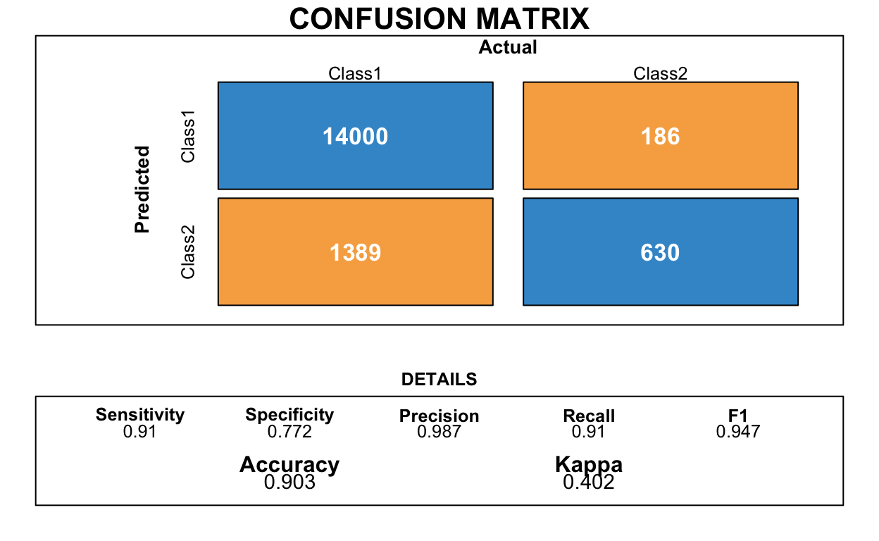
NULLThe accuracy, precision, and recall statistics for the first model are spectacular. However, the specificity statistic is not so great. The Confusion Matrix shows that a rather large number of actual Going Concern companies were predicted to be fine.
Using SMOTE sampling, the sensitivity, recall, and kappa statistics dropped by a relatively insignificant amount. The specificity statistic is much higher, though. The Confusion Matrix for this model shows that a much higher amount of the actual Going Concern companies were predicted by the model. However, the model also predicted a much higher amount of non-Going Concern companies to have that issue.
The differences between the two models displays the significance of having a sampling adjustment. SMOTE sampling essentially helps to balance the data. In this case, it attempts to balance the extreme amount of non-Going Concerns to those that are issued a Going Concern opinion.
How can this be useful?
This model could be used to help identify those companies that are more likely to have a Going Concern issue. This model could help to reduce the likelihood of a type 2 error, which is when the auditor falsely accepts the financial statements, when they should have issued a Going Concern opinion. Using the SMOTE model, an auditor can identify those companies that have a much higher likelihood of having a Going Concern issue. However, there could be a lack of efficiency due to the model identifying a decent amount of non-Going Concern companies.